OptimumCS-Pro Optical Science

There’s a great deal of lovely optical science behind OptimumCS-Pro. Feel free to ignore it — your creativity won’t suffer. If you’re interested in how the relevant quantities are calculated, though, do read on. What follows is a more detailed version of the information provided with the app.

Calculating the Optimum Focus Distance

If you know how to use a depth of field scale on a lens, you already know one method to find the optimum focus distance. The calculation presented here is mathematically equivalent to using such a scale. (Note that, although a conventional depth of field scale can give you the optimum focus distance, it CANNOT provide you with the optimum aperture.)

Imagine we’re photographing a scene that contains two objects of interest, one far away and one nearby. The images of these objects are formed at different distances behind the lens. Since we can only focus on one distance at any given time, we can’t have both objects in focus simultaneously. So what do we do? We adjust focus so that our sensor ends up half way between the images of the two objects. Neither object is then in focus, of course, but the total defocus blur that the images suffer ends up as small as possible (for the aperture we’re using), with the image blurs of the near and far objects being equal in size, And this last bit is good, because we don’t want far objects more blurry than near objects, or vice-versa.* The distance on which to focus so that our sensor is half way between the two images is given by:

Where

Clearly, u depends only on the distances to the near and far objects. Notice, also, the following familiar result:

If you’re thinking this isn’t ground breaking stuff, you’re right. And you can find a derivation of the above formula in all manner of places (e.g. Jeff Conrad’s Depth of Field in Depth, http://www.largeformatphotography.info/articles/DoFinDepth.pdf). What’s rather more interesting, and quite different from usual practice, is what comes next.

✴This is subject to debate. Ansel Adams stated that, usually, nearer objects should be given preference in terms of sharpness over further ones (The Camera, p51), while others have argued for the opposite, particularly where the horizon or objects on a distant skyline are included (e.g. Joe Englander, Apparent Depth of Field - Practical Use in Landscape Photography, http://www.englander-workshops.com/documents/depth.pdf).

Calculating the Optimum Aperture

OK, we’ve got the sensor in the right place, but it would be nice if we could make that blur smaller. We do that by stopping down the lens. As we stop down further, the blur gets smaller until, eventually, it’s so small that it no longer appears to be a blur and our picture looks sharp. A great deal of work has gone into determining just how small a blur spot needs to be before it ceases to look like a blur. Of course, if we enlarge our image sufficiently, a blur, no matter how small, will be revealed for what it. So just how small is sufficiently small, on the image formed by the lens, depends on how much we wish to enlarge that image. Now, hold those thoughts and also consider this: If we stop down the lens, we are letting less light reach the sensor. We then need either a slower shutter speed or a higher ISO, each of which can cause problems.

Optical engineers considered all this long ago, back before World War II. Back then, film was frightfully slow and most photographs were printed quite small. The question, back then, was this: What is the largest aperture that will give me a sufficiently small blur spot on a typically small print? A perfectly reasonable question. Notice that this is all about achieving barely acceptable sharpness. Stopping down further, to get sharper images, was not really much of an option when film was so slow.

So why the history lesson? Because the practices and the standards adopted by the photographic industry back in the 1930s are still with us. Depth of field scales are constructed with those standards in mind and professional photographers are trained in the same practices. There’s nothing essentially wrong with still doing things that way — if all you want is a sharp 4x5 inch print. With OptimumCS-Pro, however, we’re going to do things a little differently. We’ll concentrate on achieving the greatest possible sharpness. The Optimum approach produces far better results and is much more appropriate for the modern era of vastly improved film and high sensitivity digital sensors.

We start by recognizing something that traditional practice ignores: We can’t indefinitely continue stopping down a lens in the quest for ever greater sharpness — we reach point where stopping down further actually decreases image sharpness. This is because the effects of diffraction become increasingly bothersome at smaller apertures. Diffraction is the spreading out and resultant blurring of light that occurs when it passes through a small opening, and is quite unrelated to defocus blur.

See what’s going on? Stopping down a lens decreases defocus blur, but increases the blur due to diffraction. At some point — not too big an aperture, nor too small — there is an optimum aperture, where the combined blur due to defocus and diffraction is at its smallest.

Two pioneering articles on these matters, by Stephen Peterson and Paul Hansma, were published in Photo Techniques magazine in March/April 1996 (available from www.largeformatphotography.info/fstop.html). Peterson was interested in finding the largest aperture that would give acceptable sharpness, but went beyond standard practice by taking the effects of diffraction into account. Hansma was interested in finding the aperture that would give maximum sharpness. Although written for users of view cameras, I very highly recommend these articles — they are easy to read and contain profound ideas. Also, Conrad includes a discussion of this stuff in his paper, and that, too, is worth reading. For full background and derivations of relevant equations, you’ll need to refer to these documents. Here, I’ll simply introduce some of the key concepts and present the key results, plus a small extension to Hansma’s work so as to make it applicable to the vast majority of photographers (those who don’t use view cameras).

Let’s have a look at how Hansma proceeded.

If we use c to denote the diameter of a blur spot on our film/sensor, the diameter of the blur due to defocus is given by

where

and

This quantity, pronounced delta-v, is called the focus spread.

(all distances are measured from the lens)

The diameter of the blur due to diffraction is given by

Although the above formulae are derived through processes that involve a number of simplifying assumptions, those assumptions are quite reasonable ones and each formula is, in itself, sufficiently accurate for our purposes. But what really interests us, of course, is the diameter of a blur spot due to the combined effects of defocus and diffraction. Unfortunately, that combined blur cannot be found simply by taking the sum of the above two quantities (for many reasons). It is also worth noting that defocus blur has been calculated geometrically, while diffraction is actually due to the wave nature of light. How, then, does one combine two fundamentally different things? There is no easy answer, so Hansma made a further simplification in deciding to combine them thus:

This became

The total blur, by this construction, depends on the focus spread and on aperture. Given that N appears in the denominator of the first term and in the numerator of the second, it follows that, just as we expected, the defocus contribution decreases with f-number while the diffraction contribution increases with f-number. The blur size therefore dips to a minimum at some particular f-number. We can use differential calculus to find that f-number. Behold the result:

OK, that’s how Hansma found an expression for the optimum aperture. In comparison, a rigorous analysis, which treats all light phenomena (including defocus blur) as wave phenomena, is very much more complex than the above. If you’re interested, have a look at Conrad’s paper, where, straight after discussing Hansma’s method, he launches into a wave optics analysis, replete with Bessel functions and the like (if you don’t know what a Bessel function is, stay away)!

What’s interesting is that a rigorous wave optics analysis ultimately yields a result almost identical to Hansma’s. What’s also interesting is that Hansma actually went out and empirically tested his result and, as you can read in his magazine article, found an excellent agreement between theory and practice. And that’s fabulous news—we can have every confidence, on both theoretical and empirical grounds, that this stuff actually works very well indeed.

This formula for finding optimum aperture is perfect for view camera photography, where the photographer has direct access to, and can measure, differences in the position of the image plane (and is one of the working options available in OptimumCS-Pro). But, since most of us work in object space, we’re going to go a wee bit further and calculate the optimum aperture in terms of object distances. We’ll start by writing the optimum aperture expression thus:

Then we’ll convert image distances to object distances using well-known relationships:

and

And our optimum f-number equation becomes:

Notice that the optimum f-number depends only on the focal length and the distances to the nearest and furthest objects. Set these in OptimumCS-Pro, and the calculation is instantly performed.

Calculating Resolution

The resolution, R (in line pairs per mm), for images of the nearest and furthest objects, is given by:

(Resolution is greater for objects between these limits, reaching a maximum at focus.)

R is a measure of the sharpness of the image produced by the lens. That image is what the sensor sees. We, however, see an enlargement of that image on a computer screen or as a print. Would it not be more useful to calculate the resolution that would be achieved on such an enlargement? This is what Optimum does (and, because enlargement is involved, you’ll have to specify the width of your sensor). I’ve chosen, as a standard enlargement, one of 10 inch (250 mm) width. That’s probably the minimum size you’ll be interested in. If you go bigger, you’ll need more image resolution to start with. But, then again, maybe not, since we tend to view larger prints from greater distances. It’s up to you to make the choices.

How about a table showing what would happen if you shoot at less than the optimum f-number?

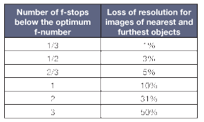
For example, let’s imagine you’re using a 24 mm lens to photograph a scene that extends from 3 m to infinity. You focus at 6 m. The optimum f-number is a bit more than f/8. If you used your lens’ depth of field scale, or a depth of field calculator, the suggested f-number would be nearly 3 stops lower. You’d lose about half your resolution for the near and far objects (actually, probably more, because lens aberrations would be rearing their ugly heads at such wide apertures).

The maximum possible resolution will be dependent on the film/sensor. It’s useful to know the maximum because, if OptimumCS’s resolution display indicates that you’re exceeding it, you can use a wider aperture if you desire. Determining resolution is a complex business, but there’s no need to go into all that. For practical purposes, all you need to do are a few simple calculations. The results will surprise most people. I’ve put this info on another page.

Accuracy

Shouldn’t we be taking lens aberrations into account? Well, no, actually. Not unless you’re using a camera with a small sensor (say, 4/3”) and wish to shoot very wide angles. For that, you’ll need an extremely short focal length lens, which will have an optimum aperture that is quite wide — close to, if not wider than the lens’ widest aperture. At such apertures, aberrations do become a problem. For all other cameras, at the sorts of apertures you’ll be using to achieve a wide depth of field, good quality lenses will have minimal aberrations. Hansma went to the trouble of testing a number of lenses and found that they performed almost exactly as his resolution formula predicts. This is good news, for it confirms what we already know from sound mathematical reasoning.

The upshot of all this is that users can be confident that OptimumCS-Pro, which is an extension into object space of mathematically sound and empirically tested methods, performs as advertised.